44 excel donut chart labels
Curved labels in Excel doughnut chart - Microsoft Community All I've seen is that you can display labels in straight lines. You can angle them, rotate them, invert them, but not curve them. You can even make them "dynamic", but no mention of curved text. The simple reality is that in terms of presentation, excel is primitive. . This article shows the label options in 2016, no mention of curves Fix label position in doughnut chart? | MrExcel Message Board Turn off data labels. Insert a Text box in to the middle of the donut, select the edge of the text box and in the formula bar hit = then select the cell that contains the progress figure. You can format this to however you want it, it will update and it won't move. Oh wow! I always thought text-boxes were just text-boxes.
Add / Move Data Labels in Charts - Excel & Google Sheets Add and Move Data Labels in Google Sheets. Double Click Chart. Select Customize under Chart Editor. Select Series. 4. Check Data Labels. 5. Select which Position to move the data labels in comparison to the bars.
Excel donut chart labels
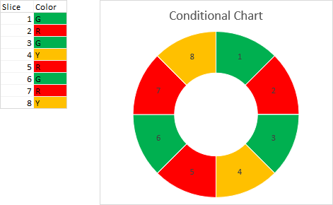
How to Rotate Pie Chart in Excel? - WallStreetMojo Move the cursor to the chart area to select the pie chart. Step 5: Click on the Pie chart and select the 3D chart, as shown in the figure, and develop a 3D pie chart. Step 6: In the next step, change the title of the chart and add data labels to it. Step 7: To rotate the pie chart, click on the chart area. Excel Doughnut Chart in 3 minutes - Watch Free Excel Video (Pie Chart ... Doughnut charts is cirular graph which display data in rings, where each ring represents a data series. In Doughnut Chart percentages are displayed in data l... Donut/Doughnut Chart - Multiple Series - Microsoft Tech Community Donut/Doughnut Chart - Multiple Series. I have created a doughnut chart with multiple series (represented by multiple rings - see charts below). Each ring is divided into 6, the colour of which corresponds to one of three options (yes, maybe and no). I therefore want the colour of the chart to represent this clearly (green, yellow and red ...
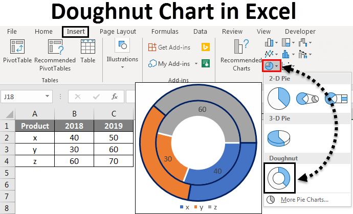
Excel donut chart labels. How to Make a Doughnut Chart in Excel | EdrawMax Online How to Make a Doughnut Chart in Excel Step 1: Input Data into the Worksheet Enable Excel 2016, open a new worksheet and input labels and data. In this example, we choose to add the data of the companies and their market shares in 2 years. Step 2: Create Your Doughnut Chart Progress Doughnut Chart with Conditional Formatting in Excel The entire chart will be shaded with the progress complete color, and we can display the progress percentage in the label to show that it is greater than 100%. Step 2 - Insert the Doughnut Chart With the data range set up, we can now insert the doughnut chart from the Insert tab on the Ribbon. The Doughnut Chart is in the Pie Chart drop-down menu. Add or remove data labels in a chart - support.microsoft.com Click the data series or chart. To label one data point, after clicking the series, click that data point. In the upper right corner, next to the chart, click Add Chart Element > Data Labels. To change the location, click the arrow, and choose an option. If you want to show your data label inside a text bubble shape, click Data Callout. Excel Charts - Doughnut Chart - tutorialspoint.com You have no more than seven categories, all of which represent parts of the whole pie. Doughnut Charts show data in rings, where each ring represents a data series. If percentages are shown in data labels, each ring will total to 100%. Doughnut charts are not easy to read. You can use a Stacked Column or Stacked Bar chart instead.
Formatting Data Label and Hover Text in Your Chart - Domo In Chart Properties , click Data Label Settings. (Optional) Enter the desired text in the Text field. You can insert macros here by clicking the "+" button and selecting the desired macro. For more information about macros, see Data label macros. (Optional) Set the other options in Data Label Settings as desired. How to add leader lines to doughnut chart in Excel? - ExtendOffice Select data and click Insert > Other Charts > Doughnut. In Excel 2013, click Insert > Insert Pie or Doughnut Chart > Doughnut. 2. Select your original data again, and copy it by pressing Ctrl + C simultaneously, and then click at the inserted doughnut chart, then go to click Home > Paste > Paste Special. See screenshot: 3. Doughnut Chart Excel | Easy Excel Tips | Excel Tutorial | Free Excel ... After adding default data labels, our example data in Doughnut Charts will look like this: Since data labels look more professional when used in percentage, we will change the default style. For this, we need to double-click on the data label or press the shortcut Ctrl + 1 after selecting any data label. Doughnut Chart in Excel - Single, Double, Format To insert the chart, follow the steps mentioned below:- Select the range of cells A2:B9 On the ribbon, move to the Insert tab. Click on the Pie Button under the Charts Group. Select the Doughnut Chart from there. This will insert a Doughnut Chart with default formatting in the current worksheet like this.
How to make doughnut chart with outside end labels? - Simple Excel VBA ... In the doughnut type charts Excel gives You no option to change the position of data label. The only setting is to have them inside the chart. But is this making You not able to make... Doughnut Chart in Excel | How to Create Doughnut Chart in Excel? - EDUCBA Now we will create a doughnut chart as similar to the previous single doughnut chart. Select the data alone without headers, as shown in the below image. Click on the Insert menu. Go to charts select the PIE chart drop-down menu. From Dropdown, select the doughnut symbol. Then the below chart will appear on the screen with two doughnut rings. Excel Doughnut chart with leader lines - teylyn Step 1 - doughnut chart with data labels Step 2 -Add the same data series as a pie chart Next, select the data again, categories and values. Copy the data, then click the chart and use the Paste Special command. Specify that the data is a new series and hit OK. You will see the new data series as an outer ring on the doughnut chart. Question: labels in an Excel doughnut chart Open your Excel document and click on your chart. In the upper bar you will find the "Diagram Tools". Click on the "Design" tab. In the "Data" group, click the "Select data" button. In the right window you will find the "Horizontal axis label". Click on "Edit". Now enter your desired names or values for the legend.
Doughnut Chart in Excel | How to Create Doughnut Chart in Excel?
Conditional Donut Chart - Peltier Tech Format the Chart. Let's do a little formatting. Double click on one of the donut slices to open the Format Data Series task pane, and under Series Options, change the Donut Hole Size from the default 75% to 50%. Click the plus icon that floats alongside the chart, and check Data Labels. Double click on one of the labels to open the Format ...
How to display leader lines in pie chart in Excel?
Curve Text in Doughnut chart - Excel Help Forum Re: Curve Text in Doughnut chart You can link WordArt to a cell using a formula. Just select the shape, click into the formula bar, type = and then select the cell and press Enter. Don Please remember to mark your thread 'Solved' when appropriate. Register To Reply 05-10-2017, 10:10 AM #5 jamesa2487 Registered User Join Date 11-20-2011 Location
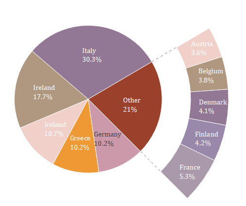
Help Online - Origin Help - Doughnut Of Pie
How to create doughnut chart in Excel? - ExtendOffice To create doughnut chart is very easy, just follow the steps: 1. Select the data range you need to be shown in the doughnut chart, and click Insert > Other Charts > Doughnut. See screenshot: In Excel 2013, click Insert > Insert Pie or Doughnut Chart > Doughnut. See screenshot: 2. Then a doughnut chart is inserted in your worksheet.

How to Make Pie Chart with Labels both Inside and Outside ...
Doughnut Chart in Excel | How to Create Doughnut Excel Chart? This article has been a guide to Doughnut Chart in Excel. We discuss creating a doughnut chart in Excel with a single data series and two data series, practical examples, and a downloadable Excel template. You may learn more about Excel from the following articles: - Types of Charts in Excel; Create a Gantt Chart in Excel; Waterfall Chart in ...

How to make a pie chart in Excel
Create Dynamic Chart Data Labels with Slicers - Excel Campus Step 6: Setup the Pivot Table and Slicer. The final step is to make the data labels interactive. We do this with a pivot table and slicer. The source data for the pivot table is the Table on the left side in the image below. This table contains the three options for the different data labels.

Doughnut Pie Chart in Excel - Infographic
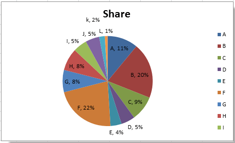
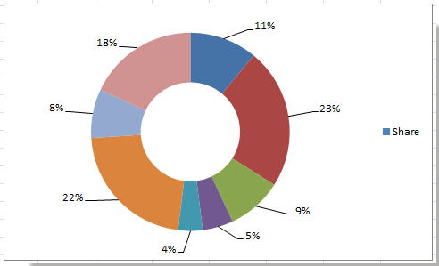
donut chart don't show all labels - Microsoft Power BI Community Because I cannot figure out why sometimes labels for the smaller values are shown and labels for larger values are not shown. e.g. in the below charts example Chart 1 all values are shown. Chart 2 I have added Germany. But the label for Columbia (2.13%) is not shown but smaller value Angola (0.92%) is shown. Message 22 of 30.
Customizing your donut chart - Datawrapper Academy
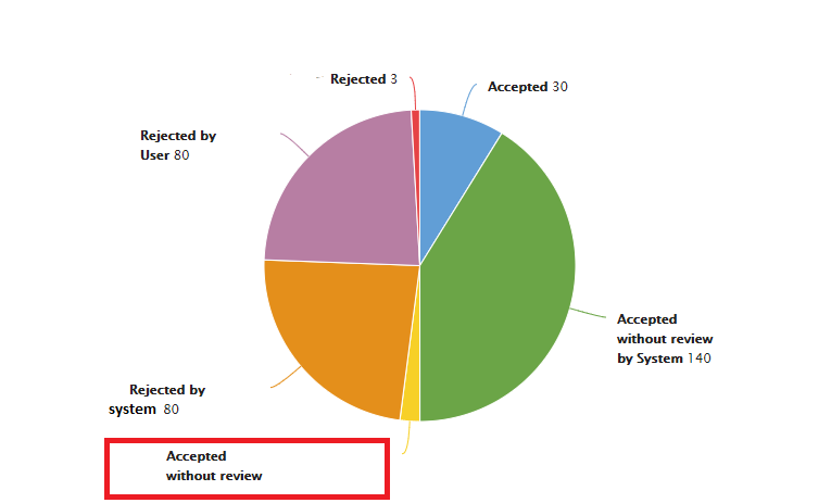
Present your data in a doughnut chart - support.microsoft.com To add text labels with arrows that point to the doughnut rings, do the following: On the Layout tab, in the Insert group, click Text Box. Click on the chart where you want to place the text box, type the text that you want, and then press ENTER.

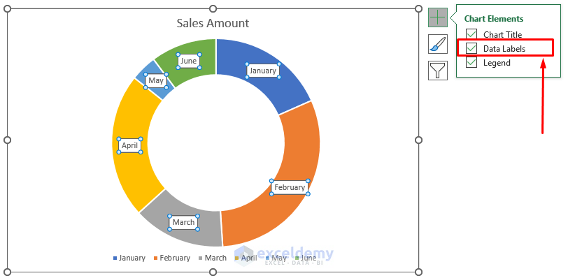
Add or remove data labels in a chart
donut chart labels - Microsoft Community To change the size of the chart, do the following: Click the chart. On the Format tab, in the Size group, enter the size that you want in the Shape Height and Shape Width box. Tip For our doughnut chart, we set the shape height to 4" and the shape width to 5.5". To change the size of the doughnut hole, do the following:
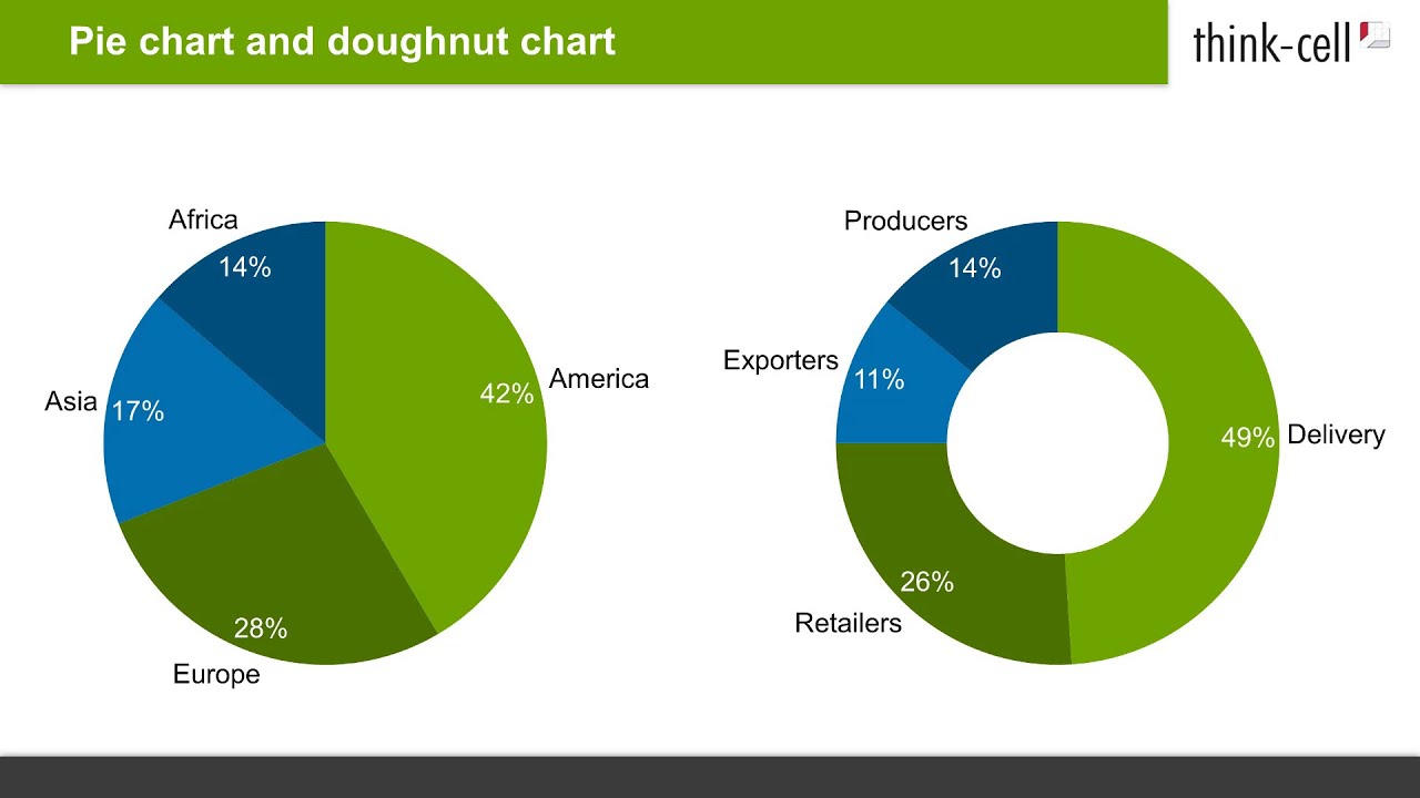
Pie chart and doughnut chart (think-cell tutorials)
Interactive Donut Chart - Beat Excel! Now select and copy the first gray area in Sheet 2 that includes blue donut part and paste it as a linked picture to cell B2 of Sheet 1. Click on this picture and type =Chart inside the formula bar. Do the same with the label but this time place it in the middle of the gray area in Sheet 1. While on Sheet 1, insert a donut chart as shown below.
Sum label inside a donut chart – amCharts 4 Documentation
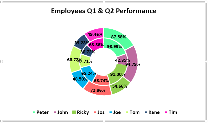
How to Create a Double Doughnut Chart in Excel - Statology Step 1: Enter the data. Enter the following data into Excel, which displays the percentage of a company's revenue that comes from four different products during two sales quarters: Step 2: Create a doughnut chart. Highlight the first two columns of data. On the Data tab, in the Charts group, click the icon that says Insert Pie or Doughnut Chart.
How to add leader lines to doughnut chart in Excel?
Donut/Doughnut Chart - Multiple Series - Microsoft Tech Community Donut/Doughnut Chart - Multiple Series. I have created a doughnut chart with multiple series (represented by multiple rings - see charts below). Each ring is divided into 6, the colour of which corresponds to one of three options (yes, maybe and no). I therefore want the colour of the chart to represent this clearly (green, yellow and red ...

How to Show Percentage in Pie Chart in Excel? - GeeksforGeeks
Excel Doughnut Chart in 3 minutes - Watch Free Excel Video (Pie Chart ... Doughnut charts is cirular graph which display data in rings, where each ring represents a data series. In Doughnut Chart percentages are displayed in data l...
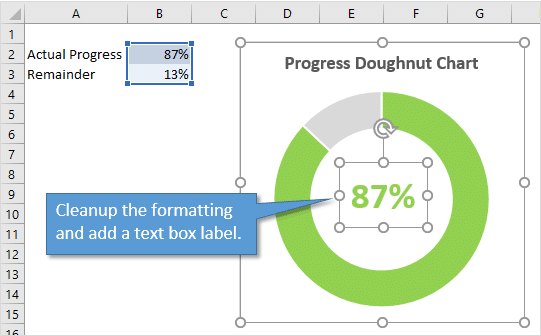
Progress Doughnut Chart with Conditional Formatting in Excel ...
How to Rotate Pie Chart in Excel? - WallStreetMojo Move the cursor to the chart area to select the pie chart. Step 5: Click on the Pie chart and select the 3D chart, as shown in the figure, and develop a 3D pie chart. Step 6: In the next step, change the title of the chart and add data labels to it. Step 7: To rotate the pie chart, click on the chart area.
How-to Make a WSJ Excel Pie Chart with Labels Both Inside and ...
Conditional Donut Chart - Peltier Tech

Inserting Data Label in the Color Legend of a pie chart ...
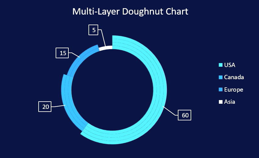
How to create a creative multi-layer Doughnut Chart in Excel

How-to Make a WSJ Excel Pie Chart with Labels Both Inside and ...

Everything You Need to Know About Pie Chart in Excel

How-to Add Label Leader Lines to an Excel Pie Chart - Excel ...

How to Create a Double Doughnut Chart in Excel - Statology

Display Total Inside Power BI Donut Chart | John Dalesandro

All about Doughnut Charts and their uses
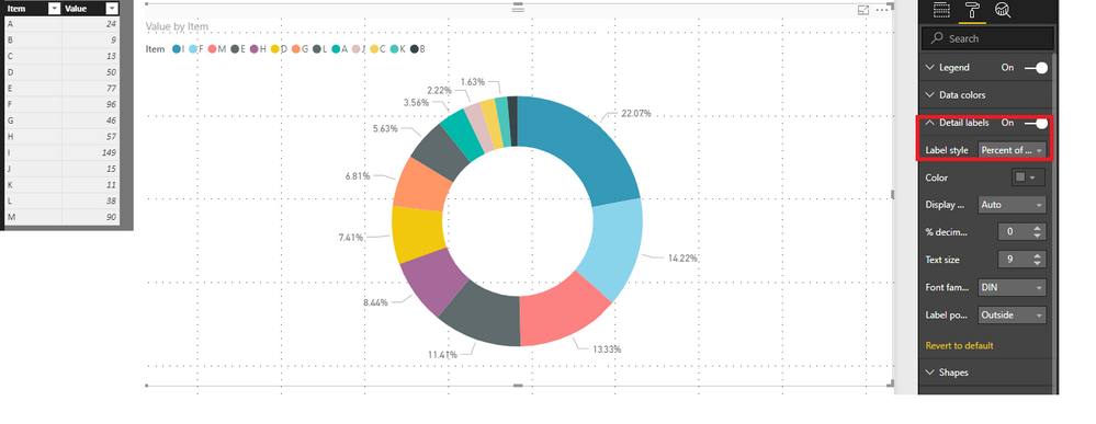
Solved: How to show all detailed data labels of pie chart ...
Curved labels in Excel doughnut chart - Microsoft Community

Best Excel Tutorial - Multi Level Pie Chart
How to Make a Doughnut Chart - ExcelNotes
Doughnut Chart in Excel | How to Create Doughnut Excel Chart?
About Doughnut Charts
Present your data in a doughnut chart

donut chart don't show all labels - Microsoft Power BI Community
/ExplodeChart-5bd8adfcc9e77c0051b50359.jpg)
How to Create Exploding Pie Charts in Excel
Remake: Pie-in-a-Donut Chart - PolicyViz
How to Create a Pie Chart in Excel | Smartsheet
5 New Charts to Visually Display Data in Excel 2019 - dummies

How to create a creative multi-layer Doughnut Chart in Excel

How to Change Excel Chart Data Labels to Custom Values?
Appian Community
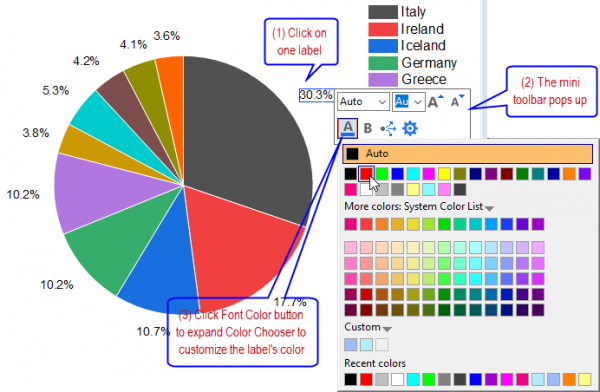
Help Online - Quick Help - FAQ-1019 How to customize the font ...

How to Make Excel Pie Chart Examples Videos ◔
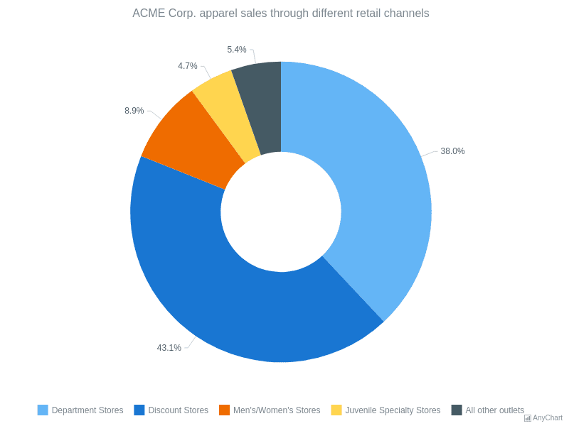
Donut Chart with Outside Labels | Pie and Donut Charts
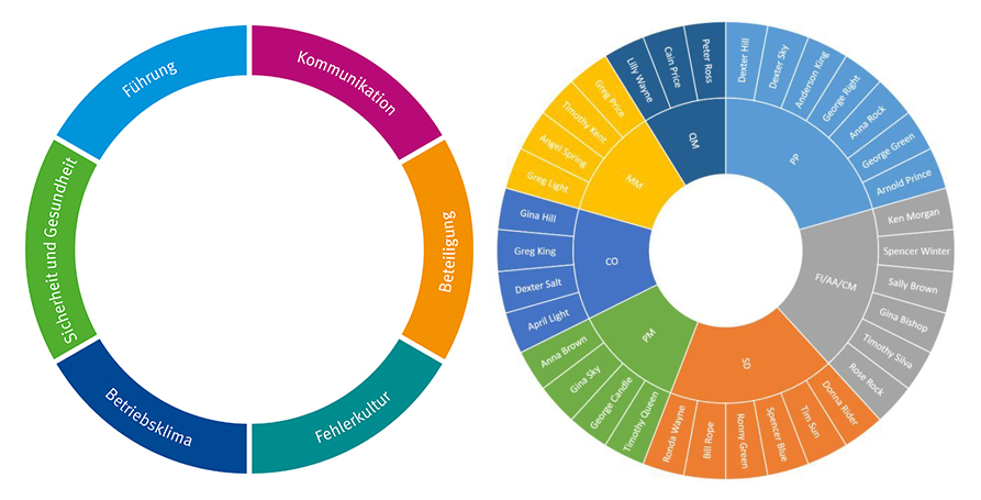
How to Create Curved Labels in Excel Doughnut Chart (With ...

How to make a pie chart in Excel
How to Create Curved Labels in Excel Doughnut Chart (With ...
Post a Comment for "44 excel donut chart labels"